GVERSE Geophysics is a seismic interpretation and analysis module that is 100% integrated with all the other GVERSE GeoGraphix modules. In GVERSE Geophysics, users can create synthetics, which are the link between well data and seismic data, allowing geological picks to be associated with reflections in the seismic data. The synthetic editing tools help users create better and cleaner synthetics to be used in the seismic interpretation. This blog will explain step-by-step how to use these synthetic editing tools.
How to manually edit synthetic curves in a seismic interpretation
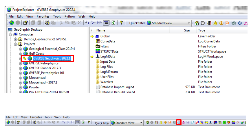
- Activate a project in GVERSE GeoGraphix and click on the GVERSE Geophysics icon on the modules tool bar.
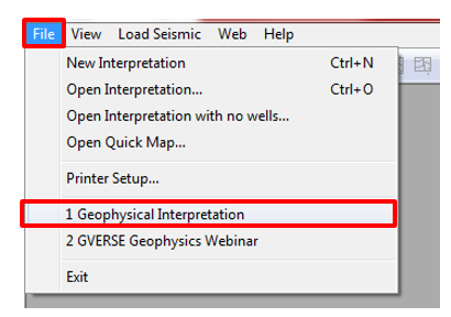
- GVERSE Geophysics will open. Go to File and select the interpretation or create a new interpretation.
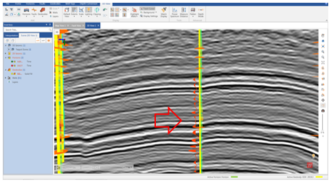
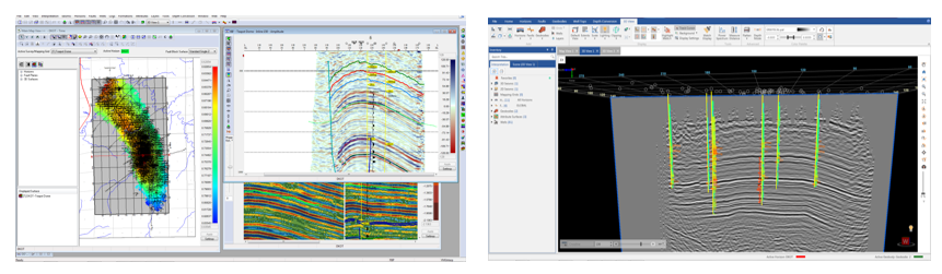
- The interpretation will open in the 2D and 3D view.
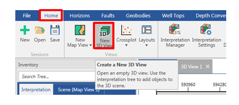
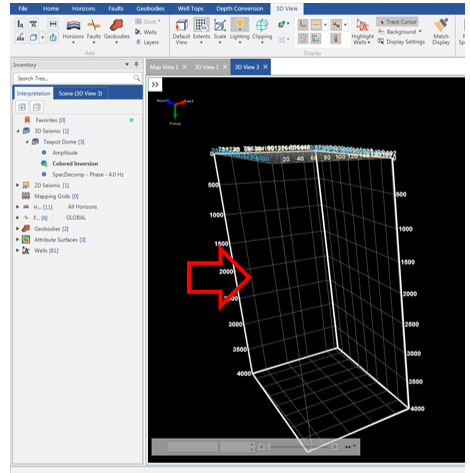
- Go to the 3D view. If you don’t have the 3D cube in the 3D view go to Home tab and click New 3D View.
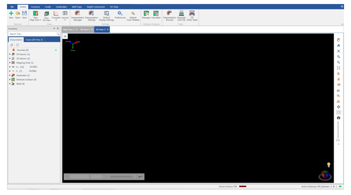
- The new 3D view tab will appear on the interpretation.
- Expand the 3D Seismic tree, select and drag the 3D version that you want to display to the black area or click the green plus-sign and Add to Scene.
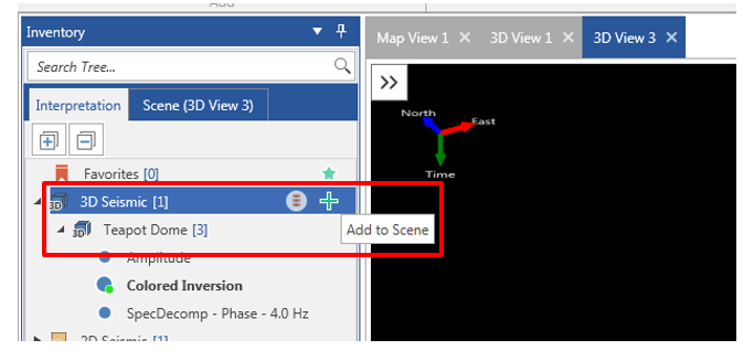
- The 3D cube will display.
- To add wells, expand the Wells tree and select the wells to be added to the view by clicking on or dragging the wells to the view. To add all the wells, click Add to Scene.
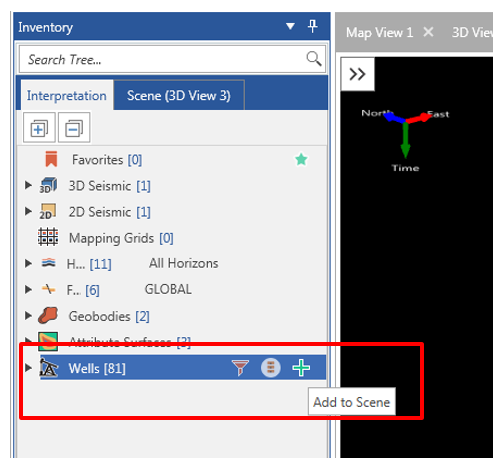
- The wells will display on the 3D view.
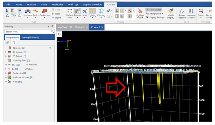
- Add the curve data for the wells if necessary.
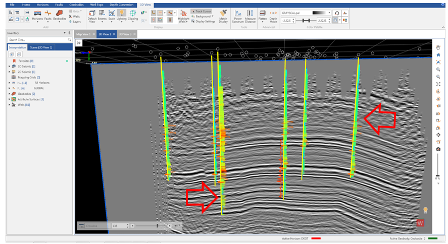
- To hilight wells with psynthetics or with sonic or density curves, go to 3D View tab and click on Highlight Wells. Select Synthetic and click Apply.
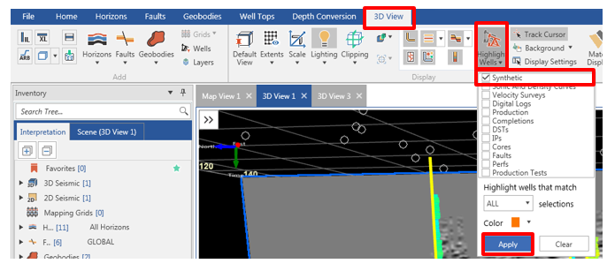
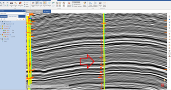
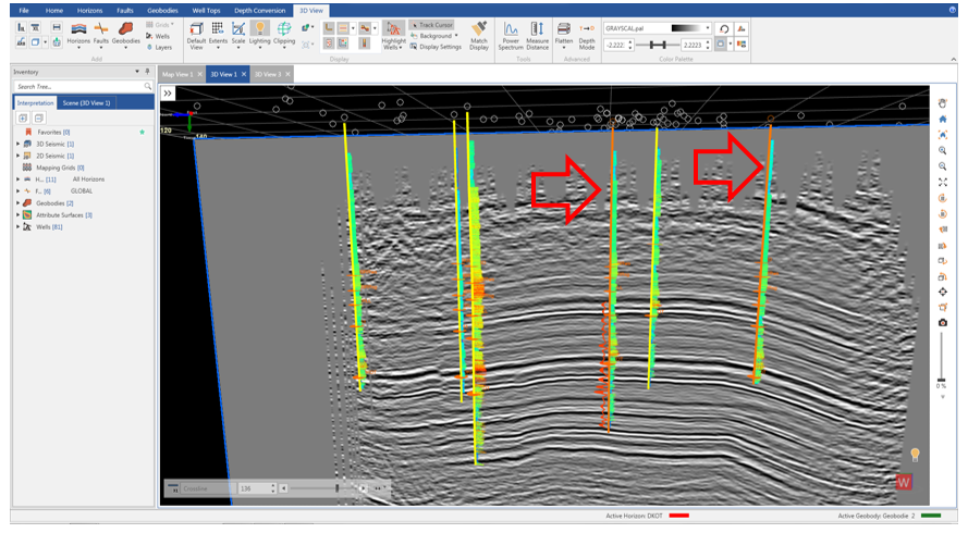
- The wells with psynthetics or with sonic or density curves will display in orange color.
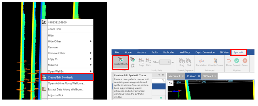
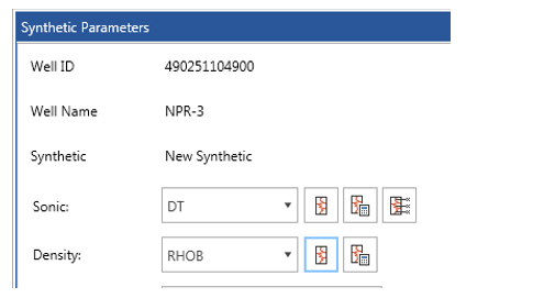
- Select a well with synthetic, right-click, and click Create/Edit Synthetic. Select the well with synthetic and on Synthetic tab click Create/Modify.
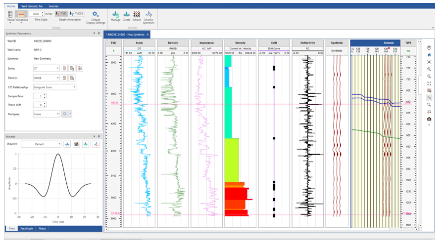
- The Create or Edit a Synthetic window will open. If you already have a synthetic in the project click OPEN SYNVIEW.
- The synthetic will display.
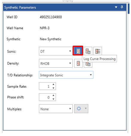
Sonic: Log Curve Processing Tool
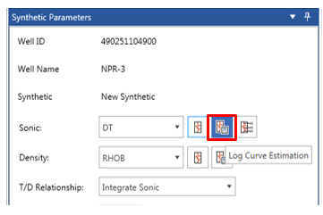
- On the Synthetic Parameters go to Sonic and click on Log Curve Processing.
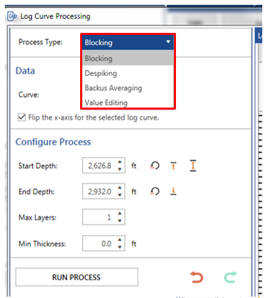
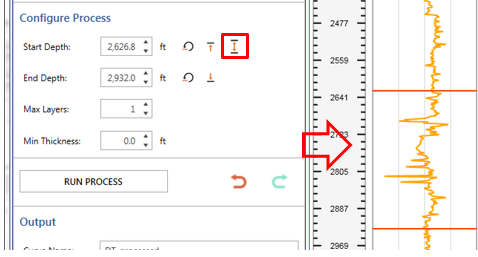
- The Log Curve Processing window will open. In Process Type select between Blocking, Despiking, Backus Averaging, and Value Editing. In Configure Process select the parameters. You can select a specific depth range in the log from the depth range tool >> select the window in the log. Click Run Process.
- Two new tracks will appear: Processed and Comparison . The purple curve is the processed curve.
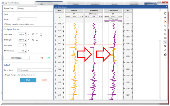
- Use the other Process Type and select the paramaters if necessary to obtain better results.
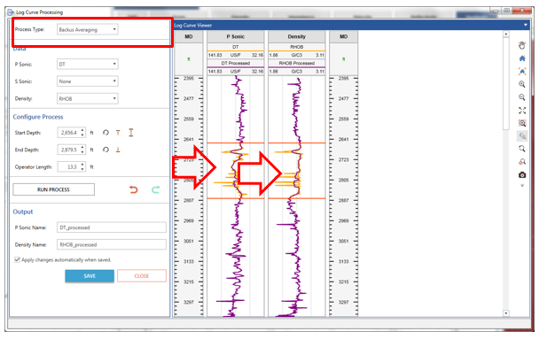
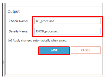
- If you are happy with the results on Output add a name and click Save.
Sonic: Log Curve Estimation Tool
- Go back to Synthetic Parameters and in Sonic click Log Curve Estimation.
- The Log Curve Estimation window will open.
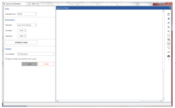
- In Parameters go to Estimate and select Sonic from Density or Density From Sonic.
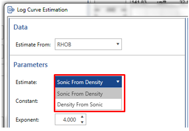
- Select the Constant and the Exponent and click ESTIMATE CURVE. A new estimated track will appear in purple.
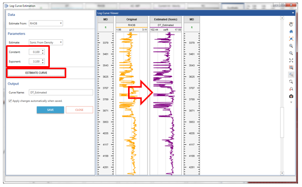
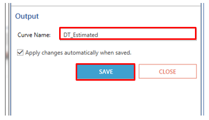
- In Output add a new name in Curve Name and click SAVE.
Sonic: Sonic Calibrations Tool
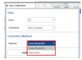
- In Synthetic Parameters click Sonic Calibration.
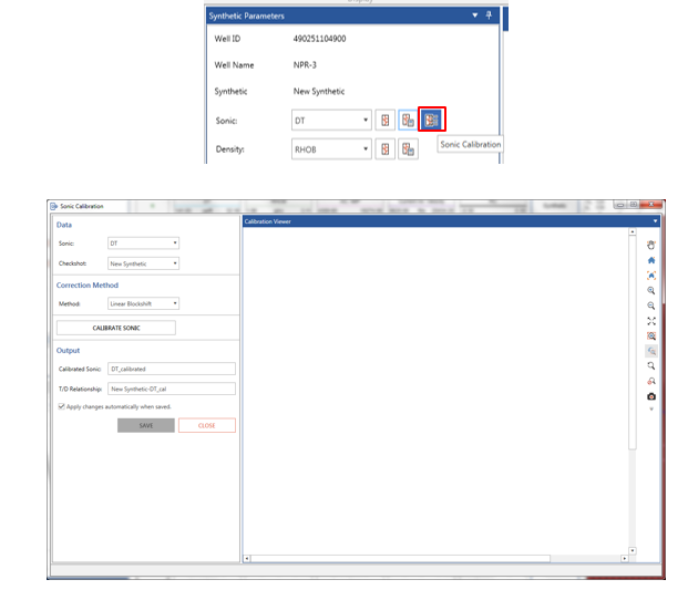
- In the Sonic Calibration window, under Data select Sonic and Checkshot. Under Correction Method select Linear Blockshift or Polynomial. If you select Polynomial select the order. Click CALIBRATE SONIC.
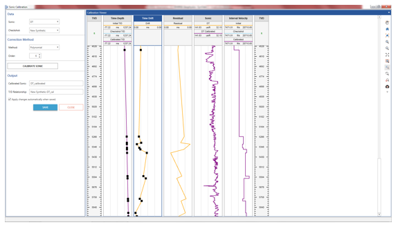
- The Time Drift or/and Residual track will appear and the calibrated curve will display in purple.
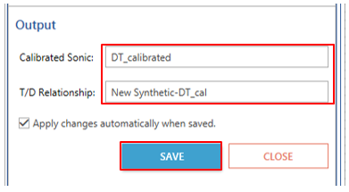
- In Output add new and click SAVE.
- The same steps can be followed for density curve (Log Curve Processing & Log Curve Estimation).
- After finishing save all the changes and close the synthetic window.
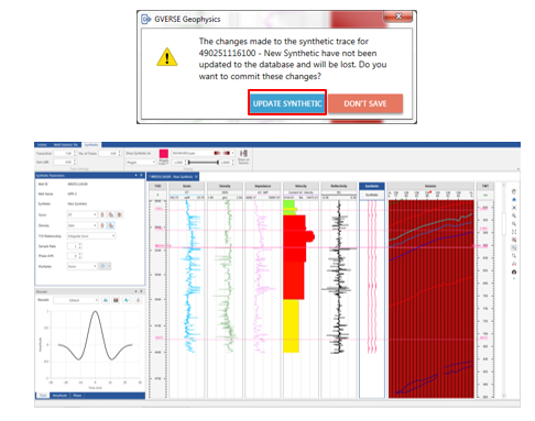
- The changes will be applied to the interpretation.